


쿠팡파트너스 활동으로 수수료를 제공받을 수 있습니다.
Nelson-Siegel 모형
Yield Curve, Volatility Term Structure Modeling 등에 이용되는 모형 중 하나로, Monotone, Humped, S shape의 커브를 표현
Parsimonious Model


적은 갯수의 parameter가 데이터를 잘 설명한다는 의미.
적은 갯수의 parameter를 쓰는 simple한 모델이 주어진 데이터를 잘 설명할때, Parsimonious Model이라함.
파라미터 갯수를 많이 쓰는 모델은 설명력이 좋을 수 있으나, 파라미터 추정이 어려워서 실무적 활용이 어려울 수 있다.
오컴의 면도날에서 말하듯이, 같은 현상을 설명하는, 설명력이 비슷하다면, 단순한게 최고.
Abstract
본문에서는,
Monotone, Humped, S shape의 Yield curve를 표현할 수 있는 기능을 갖추고 있는 parametric model로, parametrically parsimonious 한 모델을 소개함.
1981~1983년 기간동안 YTM에 적용해봤을때 YTM variation의 96%를 설명함.
시간에 따라 변하는 parameter 값은, 1982년 말 연준의 통화정책 변화와 관련된 YTM 변동도 반영한다.
모델에서 얻는 Fitting curve는 Long Term Treasury bond의 Price를 0.96의 correlation으로 예측하는데, 모델은 수익률/만기 관계의 중요한 속성을 포착하고 있음.
1. Introduction
The fitting of yield curves to yield/maturity
•
David Durand (1942)이 선구자. 분산된 포인트들 하에서 Monotonic Envelope를 그리는 방법을 시도
•
J. Huston McCulloch (1971, 1975): Yield → 현가. 가격 데이터에 맞는 piecewise polynomial spline으로, 현가를 근사
•
Gary Shea(1982, 1985): 수익률 함수가 표본에서 관찰된 maturity 범위의 끝 부분으로 갈수록 급격하게 구부러지는 경향이 있음을 보임.
이 연구에서의 결과는, 모델이 샘플의 maturity 범위를 벗어난 예측, 즉 샘플 데이터에 존재하는 가장 긴 만기 보다 더 긴 만기의 Yield를 모델로 설명하는 것은 유용하지 않다고함.
•
Cohen, Kramer, Waugh(1966), Fisher(1966), Echols 및 Elliott(1976), Dobson(1978), Heller 및 Khan(1979), Chambers
다양한 매개변수 모델을 수익률 곡선에 적용하려는 시도.
→ Polynomial regression based model(Polynomial spline) / Exponential Spline으로 근사해보려 함
→ 두 방법 모두 샘플 데이터에 존재하는 만기 내에서는 잘 피팅 됐지만, 그 보다 긴 만기의 rate를 추정하기 위해 커브를 외삽 할 땐, rate가 unboundedly large하게 나타남.
YTM : Average of instantaneous forward rate
본문에서의 YTM은 YTM on bill. T-bill은 Zero Coupon bond이므로, YTM과 Spot rate는 같다. 따라서, 여기서의 YTM은 Spot rate를 의미한다.
첫번째 모델 가정: 5개의 Parameter
maturity 인 instantaneous forward rate 에 대해 아래의 equation 만족한다고 가정해보자.
Model parameters
: time constant associated with equation
: determined by initial conditions → forward curve의 monotone, hump, S 쉐입 결정
Standard Software로 모델 추정 해보는데 수렴에 실패하더라… 매개변수 갯수가 너무 많다(overparameterized)
두번째 모델 (More Parsimonious model): 4개의 Parameter
두번째로 가정하는 모델이 “넬슨-시겔 모형”으로 익히 알려진 모형이다.
Forward rate
YTM
상수 + Laguerre function 의 형태로 볼 수 있음
Laguerre function: 다항식 * exeponential decay term으로 구성됨
주어진 coefficient 에 대해서 Linear함.
필연적으로 은 의 평균과 같기 때문에,
m이 커짐에 따라 R(m)의 Limit 값은 , m이 작아짐에 따라 R(m)의 Limit 값은 이다.
일때는, 에 적용될 수 있는 shape의 범위는 Single parameter에 의존한다.
이므로, 라는 파라미터 한가지에 의해 컨트롤된다.
→ 값을 -6 ~ 12 사이에서 동일한 증분값을 주면서 움직여보면, YTM curve는 Fig 1 처럼 움직임. (Monotone, Humped, S커브 등의 shape을 볼 수 있다)
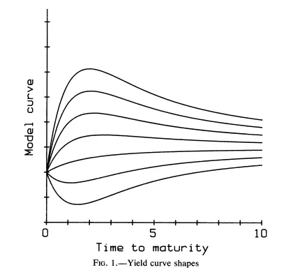
모델의 shape flexibility
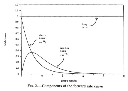
Level : long-term component에 기여하는 파라미터. (0으로 decay 하지 않는 상수)
Slope 로 묶이는 term: short-term component에 기여 (0으로 가장 빠르게 감소하는 항)
Hump 으로 묶이는 term: medium-term component에 기여(0에서 시작(not short-term), 0으로 감소하는 항)
Nelson-Siegel: Level, Slope, Hump 요소의 합으로 커브 표현
각 구성 요소에 대하여 적절한 가중치 선택으로 monotone, humped, S shape을 만들 수 있음.
모수 추정 방법
Nonlinear Least Square: Levenberg-Marquardt algorithm
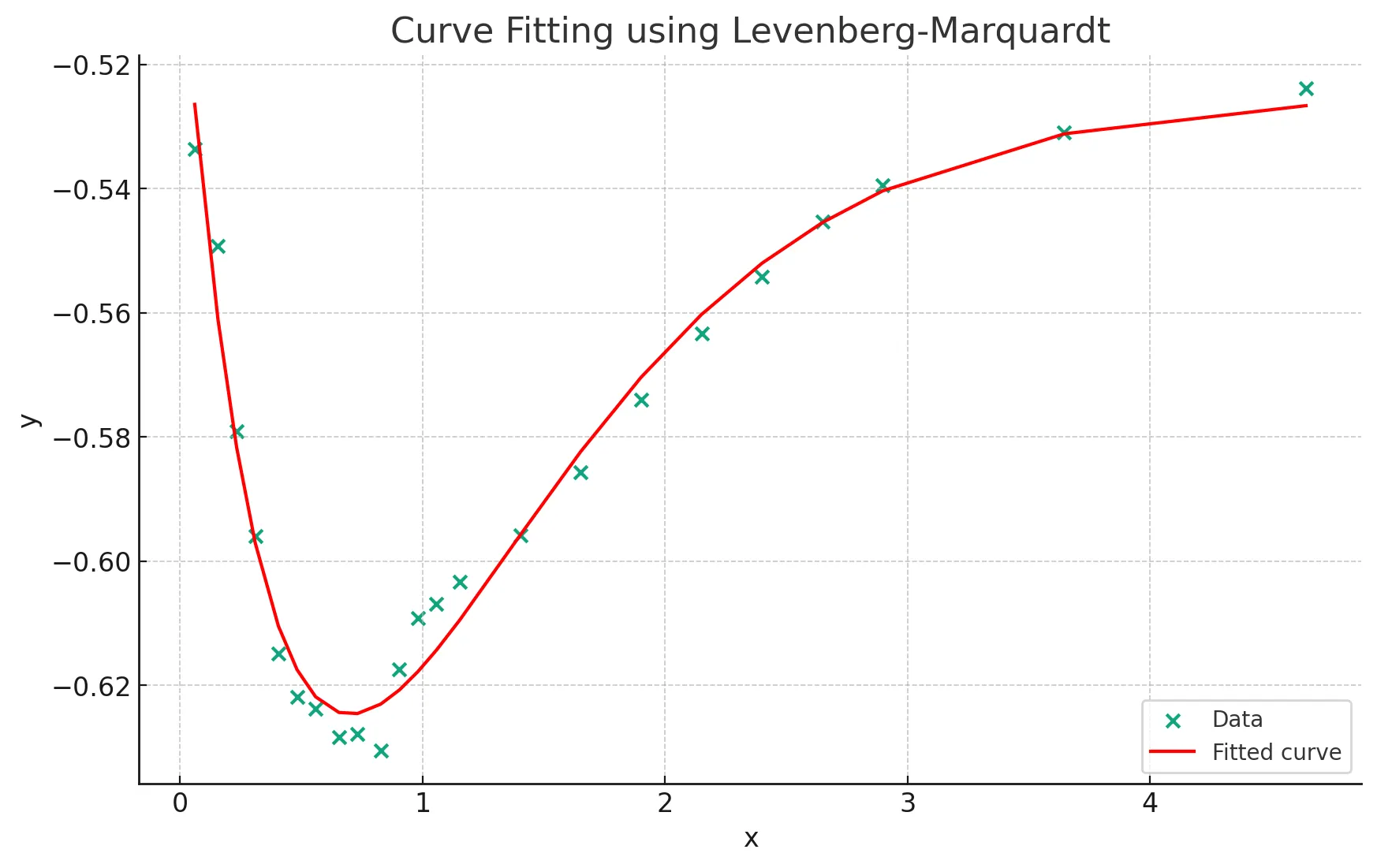
Levenberg-Marquardt를 이용한 Curve Fitting 예시
23개의 (x,y) 데이터가 주어졌을때,
Short term component , Mid term component , Long term component
를 모델링하는 Fitting function 에 데이터를 fitting해보자.
(주어진 데이터의 분포를 보았을때, Hump를 모델링하는 항이 있어야 Fitting이 잘됨)
에 대하여, 초기값은 , Upper Boundary와 Lower Boundary는 각각 와 로 주고,
function evaluate의 횟수는 max 5000번으로 두고 Leverberg-Marquardt를 돌렸다.
import numpy as np
from scipy.optimize import curve_fit
import matplotlib.pyplot as plt
# Define the model function
def model(x, p1, p2, p3, p4, p5):
return p1 + p2 * np.exp(p3 * x) + p4 * x * np.exp(p5 * x)
# Given data points
x_data = np.array([
0.0602739726027397, 0.156164383561644, 0.232876712328767, 0.309589041095890,
0.405479452054795, 0.482191780821918, 0.558904109589041, 0.654794520547945,
0.731506849315069, 0.827397260273973, 0.904109589041096, 0.980821917808219,
1.05753424657534, 1.15342465753425, 1.40273972602740, 1.65205479452055,
1.90136986301370, 2.15068493150685, 2.40000000000000, 2.64931506849315,
2.89863013698630, 3.64657534246575, 4.64383561643836
])
y_data = np.array([
-0.5335983478, -0.5492093171, -0.5791168148, -0.5959905128, -0.6148176477,
-0.6219066091, -0.6237523337, -0.6283676619, -0.6278733227, -0.6305144539,
-0.6174757245, -0.6091777567, -0.6068296497, -0.6033343905, -0.5958034148,
-0.5856756984, -0.5739923325, -0.5633682932, -0.5542019703, -0.5453668113,
-0.539440631, -0.5309504566, -0.5238687851
])
# Initial parameter guesses and bounds
initial_guess = [0, 1, -1, 0, -1] # These are arbitrary and might need tuning
bounds = ([-np.inf, -np.inf, -np.inf, -np.inf, -np.inf], [np.inf, np.inf, np.inf, np.inf, np.inf])
max_fev = 5000 # Max number of function evaluations, updated as per your request
# Perform the curve fitting
popt, pcov = curve_fit(model, x_data, y_data, p0=initial_guess, bounds=bounds, maxfev=max_fev)
# Print the optimal parameters
print("Optimal parameters (p1*, p2*, p3*, p4*, p5*):", popt)
# Plot the original data and the fitted curve
plt.scatter(x_data, y_data, label='Data')
plt.plot(x_data, model(x_data, *popt), label='Fitted curve', color='red')
plt.xlabel('x')
plt.ylabel('y')
plt.title('Curve Fitting using Levenberg-Marquardt')
plt.legend()
plt.show()
Python
복사
Optimal parameters (p1*, p2*, p3*, p4*, p5*): [-0.52484216 0.02636295 -3.44200381 -0.41812805 -1.50363265]